Shrinkage Methods

Shrinkage methods are regression methods that estimate the coefficients by constraining or penalizing their size. The main idea is to allow a small amount of bias in exchange for a potentially large reduction in variance, which can improve out-of-sample prediction.

In ordinary linear regression, the OLS estimator minimizes the residual sum of squares,

$$\mathrm{RSS}(\beta )=\Vert Y-X\beta {\Vert }_2^2.$$

When there are many predictors, when the predictors are highly correlated, or when the signal is weak relative to the noise, OLS can have high variance and can overfit the training data. Shrinkage methods address this by pulling the estimated coefficients toward zero.

Definition

A shrinkage method modifies the least-squares objective by adding a penalty on the size of the coefficients.

Intuition

Large coefficients allow the model to fit the training data more aggressively. Penalizing coefficient size discourages overly complex fits and can make the model more stable under small changes to the data.

This is closely related to model selection, but it is not exactly the same thing.

1. Model selection usually compares several candidate models and chooses one.
2. Shrinkage keeps all predictors in a single optimization problem, but penalizes them so that the fitted model becomes less flexible.
3. In practice, the amount of shrinkage is usually chosen by cross-validation.

The tuning parameter is usually denoted by $\lambda \ge 0$.

1. If $\lambda =0$, we recover the usual least-squares solution.
2. As $\lambda$ increases, the coefficients are shrunk more strongly toward zero.
3. If $\lambda$ is too large, the model can underfit.

Warning

Since the penalty depends on the scale of the coefficients, shrinkage methods are usually applied after standardizing the predictors. Otherwise, predictors measured on larger scales may be penalized differently for purely unit-related reasons.

Ridge Regression

Ridge regression adds an $L_2$ penalty to the least-squares objective:

$${\hat{\beta }}^{\mathrm{ridge}}={\mathrm{argmin}}_{\beta }\left\{\Vert Y-X\beta {\Vert }_2^2+\lambda \sum _{j=1}^p{\beta }_j^2\right\}.$$

Equivalently, ridge regression can be written in constrained form as

$${\mathrm{argmin}}_{\beta }\Vert Y-X\beta {\Vert }_2^2\text{subject to}\sum _{j=1}^p{\beta }_j^2\le t$$

for some $t\ge 0$.

Here the penalty is placed on the non-intercept coefficients; the intercept is usually not penalized.

If $X^{\mathrm{T}}X$ is invertible, the ridge estimator has the closed form

$${\hat{\beta }}^{\mathrm{ridge}}=(X^{\mathrm{T}}X+\lambda I{)}^{-1}{X}^{\mathrm{T}}Y.$$

Intuition

Ridge regression keeps the least-squares objective but adds a cost for large coefficients. The optimizer therefore prefers solutions with smaller coefficient magnitudes, especially in directions where the data do not strongly identify the coefficients.

Important properties:

1. Ridge shrinks coefficients continuously toward zero, but typically does not set them exactly equal to zero.
2. It is especially helpful when predictors are highly correlated, since OLS can become unstable in that setting.
3. It reduces variance at the cost of introducing bias.
4. The fitted model still uses all predictors, so ridge is usually not viewed as a variable selection method.

Interpretation

Ridge is often preferred when many predictors each carry a little signal, rather than when only a small subset is truly important.

Lasso Regression

The lasso adds an $L_1$ penalty to the least-squares objective:

$${\hat{\beta }}^{\mathrm{lasso}}={\mathrm{argmin}}_{\beta }\left\{\Vert Y-X\beta {\Vert }_2^2+\lambda \sum _{j=1}^p|{\beta }_j|\right\}.$$

Equivalently, the constrained form is

$${\mathrm{argmin}}_{\beta }\Vert Y-X\beta {\Vert }_2^2\text{subject to}\sum _{j=1}^p|{\beta }_j|\le t.$$

As with ridge, the intercept is usually not penalized.

Intuition

The lasso penalizes the absolute values of the coefficients, so increasing a coefficient away from zero has a constant marginal penalty rather than a smoothly increasing quadratic penalty. This makes zero a particularly attractive solution for some coefficients.

Important properties:

1. The lasso shrinks coefficients toward zero.
2. Unlike ridge, it can set some coefficients exactly equal to zero.
3. Because of this, the lasso performs a form of automatic variable selection.
4. When predictors are highly correlated, the lasso may select one and ignore others, which can make the selected model less stable.

Interpretation

The lasso is often useful when you believe that only a relatively small subset of predictors is truly needed.

Differences Between Ridge and Lasso Regression

The two methods differ in both behavior and geometry.

High-Level Comparison

1. Ridge uses an $L_2$ penalty, ${\sum }_j{\beta }_j^2$.
2. Lasso uses an $L_1$ penalty, ${\sum }_j|{\beta }_j|$.
3. Ridge usually keeps all predictors in the model, but with smaller coefficients.
4. Lasso can set some coefficients exactly to zero and therefore acts as a variable selection method.

Why Does Lasso Encourage Sparsity?

The cleanest way to see the difference is through the constrained formulations.

For ridge, the constraint region is

$$\sum _{j=1}^p{\beta }_j^2\le t,$$

which is a smooth ball. For the lasso, the constraint region is

$$\sum _{j=1}^p|{\beta }_j|\le t,$$

which has corners aligned with the coordinate axes.

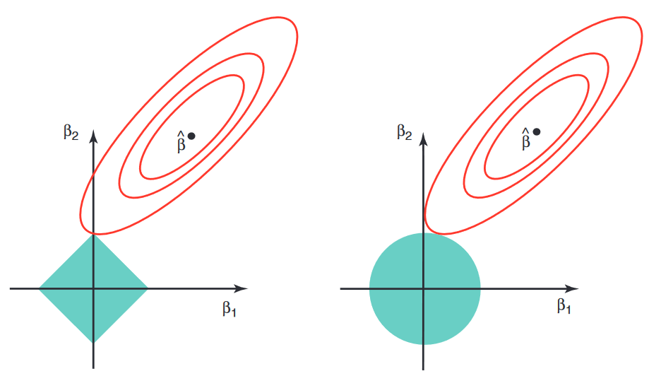
Geometric Intuition

The least-squares objective has elliptical level sets. The solution occurs where the smallest such ellipse first touches the constraint region. A smooth ridge ball is usually touched away from the axes, so the coefficients are shrunk but not forced to zero. The lasso region has sharp corners on the axes, and the ellipse often touches one of those corners, which corresponds to one or more coefficients being exactly zero.

There is also an optimization viewpoint. The ridge penalty is differentiable:

$$\frac{d}{d{\beta }_j}{\beta }_j^2=2{\beta }_j.$$

Near zero, this derivative is also near zero, so the penalty does not create a special pull to make a coefficient exactly zero.

By contrast, the lasso penalty involves $|{\beta }_j|$, which has a kink at zero. Away from zero,

$$\frac{d}{d{\beta }_j}|{\beta }_j|=\{\begin{array}{ll}1& {\beta }_j>0\\ -1& {\beta }_j<0.\end{array}$$

At zero, the derivative is not unique; informally, zero is a special point where the penalty can keep a coefficient pinned at exactly zero unless the data provide enough evidence to move it away.

Practical Tradeoffs

Reasons to prefer ridge:

1. Many predictors have small or moderate effects.
2. Predictors are strongly correlated.
3. Prediction accuracy matters more than model sparsity.

Reasons to prefer lasso:

1. You expect only a relatively small number of predictors to matter.
2. You want an interpretable sparse model.
3. Variable selection is part of the goal.

Warning

The lasso can be unstable when several predictors are highly correlated, since it may arbitrarily prefer one over another. Ridge tends to spread the effect more smoothly across correlated predictors.

Interview Summary

Ridge shrinks coefficients continuously but usually keeps them nonzero. Lasso uses an $L_1$ penalty with axis-aligned corners, so the optimum often lands exactly on one or more axes, which is why it encourages sparsity and performs variable selection.