Generative Adversarial Networks

A generative adversarial network or GAN is an unsupervised model that aims to generate new samples that are indistinguishable from a set of training examples. GANs are just mechanisms to create new samples; they do not build a probability distribution over the modeled data and hence cannot evaluate the probability that a new data points belongs to the same distribution.

In a GAN, the main generator network creates samples by mapping random noise to the output data space. If a second discriminator network cannot distinguish between the generated samples and the real examples, the samples must be plausible. If this network can tell the difference, this provides a training signal that can be fed back to improve the quality of the samples.

Caution

The idea is simple, but training GANs is difficult: the learning algorithm can be unstable, and although GANs may learn to generate realistic samples, this does not imply that they learn to general all possible samples.

Discrimination as a Signal

We aim to generate new samples that are drawn from the same distribution as a set of real training data . A single new sample is generated by

1. choosing a latent variable from a simple base distribution (e.g. a standard Normal), and
2. passing this through a generator network with parameters .

During the learning process, the goal is to find parameters so that the samples look similar to the real data . Similarity can be defined in many ways, but the GAN uses the principle that the samples should be statistically indistinguishable from the true data. To this end, a second network is called the discriminator is introduced. This network aims to classify its input as being a real example or a generated sample.

GAN Loss Function

The discriminator takes input , has parameters , and returns a scalar that is higher when it believes the input is a real example. This is a binary classification task, so we adapt the binary cross-entropy loss function. In this case, we assume that the real examples have label and the generated samples have label so that

where and index the real examples and generated examples respectively. Now we substitute the definition for the generator and note that we must maximize with respect to since we want the generated samples to be misclassified

Training GANs

The above equation is complex, the discriminator parameters are manipulated to minimize the loss function, and the generative parameters are manipulated to maximize the loss function. GAN training is characterized as a minimax game; the generator tries to find new ways to fool the discriminator, which in turns searches for new ways to distinguish generated samples from real examples. If training proceeds as planned, then upon convergence, will be drawn from the same distribution as the data, and will be at chance (i.e. 0.5).

To train the GAN, we can divide the above Equation 2 into two loss functions:

where we multiplied the second function by minus one to convert to a minimization problem and dropped the second term, which has no dependence on . Minimizing the first loss function trains the discriminator, and minimizing the second trains the generator.

At each step, we draw a batch of latent variables from the base distribution and pass these through the generator to create samples . Then we choose a batch of real training examples . Given the two batches, we can now perform one or more gradient descent steps on each loss function.

Deep Convolutional GAN

The deep convolutional GAN or DCGAN was an early GAN architecture specialized for generating images. The input to the generator is a 100D latent variable sample from a uniform distribution. This is then mapped to a spatial representation with 1024 channels using a linear transformation. Four convolutional layers, each of which use a fractionally-strided convolution that doubles the resolution (i.e. a convolution with a stride of 0.5). At the final layer, the signal is passed through a function to generate an image in the range . The discriminator is a standard convolutional network where the final convolutional layer reduces the size to with one channel. This single number is passed through a sigmoid function to create the output probability.

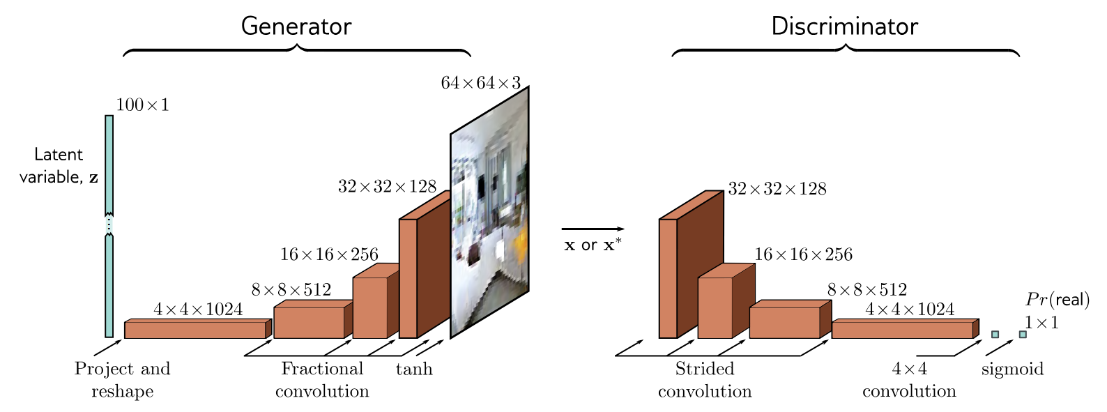
After training, the discriminator is discarded. To create new sampled, latent variables are drawn from the base distribution and passed through the generator.

Difficulty in Training GANs

Theoretically, training a GAN is straightforward. However, GANs are notoriously difficult to train. For example, to get the DCGAN to train reliably, it was necessary to use

• use strided convolutions for upsampling and downsampling
• BatchNorm layers in both the generator and discriminator except in the last and first layers, respectively
• use the leaky ReLU activation function in the discriminator, and
• use the Adam optimizer but with a lower momentum coefficient than usual.

This is unusual, as most deep learning models are relatively robust to such choices. A common failure mode is that the generator makes plausible samples, but these only represent a subset of the data (e.g. for faces, it might never generate faces with beards). This is known as mode dropping. An extreme version of this phenomenon can occur where the generator entirely or mostly ignores the latent variables and collapses all samples to one or a few points. This is known as mode collapse.

Improving Stability

To understand why GANs are difficult to train, it is necessary to understand exactly what the loss function represents.

Analysis of GAN Loss Function

The instability does not come from the algebra itself. It comes from what the algebra says the generator is optimizing after the discriminator has become good. To see this, divide the two sums in Equation 3 by the numbers , of real and generated samples, so the discriminator loss can be written as expectations:

where is the probability distribution over the generated samples, and is the true probability distribution over real examples.

When , the optimal discriminator for an example of unknown origin is

where on the right hand side, we evaluated against the generated distribution and the real distribution . Substituting back into Equation 5,

Disregarding additive and multiplicative constants, this is the Jensen-Shannon divergence between the synthesized distribution and the true distribution .

The first term is small if, whenever the sample density is high, the mixture is also high. In other words, it penalizes generated samples in regions where there are no real examples; it enforces quality. The second term is small if, whenever the true density is high, the mixture is also high. In other words, it penalizes real examples in regions where there are no generated samples; it enforces coverage.

This sounds reassuring: minimizing the Jensen-Shannon divergence should push the generated distribution toward the data distribution. The problem is that this statement assumes an optimal discriminator and says little about whether gradient descent gives the generator a useful direction at each finite training step.

Suppose the generator currently puts probability mass in the wrong region of the data space. Then and may have little or no overlap, especially in high-dimensional spaces like images. In those regions the optimal discriminator is nearly perfect:

Once this happens, the discriminator tells the generator only “this is fake,” not which direction would make it more real. The Jensen-Shannon divergence has essentially saturated: moving a generated sample a small distance may not change whether it lies in the support of the real data, so the loss can remain almost constant. A nearly constant loss means a nearly useless gradient for the generator.

Intuition

The discriminator is useful only when it is imperfect in an informative way. If it is too weak, its gradients do not identify what makes samples unrealistic. If it is too strong, it classifies generated samples as fake with near certainty, and the generator receives little information about how to move toward the data distribution. GAN training is therefore unstable because the learning signal depends on keeping the discriminator in a narrow useful regime.

This also helps explain mode dropping. The generator loss in Equation 4 is evaluated only on generated samples. It strongly penalizes generated samples that look fake, but it does not directly sample missing regions of the true data distribution and say “generate something here too.” Coverage pressure comes indirectly through the discriminator, and that signal can vanish or become noisy when the discriminator separates real and generated samples too easily. As a result, the generator can reduce its loss by producing a smaller set of realistic samples rather than covering every mode of the data distribution.

Vanishing Gradients

The original minimax generator loss is

If the discriminator confidently recognizes generated samples, then . In that case the generator is optimizing near . Because the discriminator output is already saturated near zero, changing only weakly changes the loss, so the generator gradient can vanish.

This is why GAN implementations often use the non-saturating generator loss

This objective has the same preferred solution, but gives a much larger gradient when the discriminator assigns low probability to generated samples. It does not remove the minimax instability, but it makes early training less likely to stall.

TODO

• Add various GAN architectures: StyleGAN, CycleGAN, Pix2Pix, InfoGAN, ConditionalGAN
• Wasserstein GAN loss

Sources

• Prince, S. (2023). Understanding Deep Learning. Chapter 15.j
• Unsupervised Representation Learning with Deep Convolutional Generative Adversarial Networks