Normalizing Flows

Normalizing flows learn a probability model by transforming a simple distribution into a more complicated one using a deep network. Normalizing flows can both sample from this distribution and evaluate the probability of new examples. However, they require specialized architecture: each layer must be invertible. In other words, it must be able to transform data in both directions.

1D Case

Consider modeling a 1D distribution . Normalizing flows start with a simple tractable base distribution over a latent variable and apply a function , where the parameters are chosen so that has the desired distribution. Generating a new example is easy: we draw from the base density and pass this through the function so that .

Measuring Probability

Measuring the probability of a data point is more challenging. Consider applying a function to random variable with known density . The probability density will decrease in areas that are stretched by the function and increase in areas that are compressed so that the area under the new distribution remains one. The degree to which a function stretches or compresses its input depends on the magnitude of its gradient. If a small change to the input causes a larger change in the output, it stretches the function. If a small change to the input causes a smaller change in the output, it compresses the function.

More precisely, the probability of data under the transformed distribution is

where is the latent variable that created . The term is the original probability of this latent variable under the base density. This is moderated according to the magnitude of the derivative of the function. If this is greater than one, then the probability decreases. If its smaller, the probability increases.

Forward and Inverse Mapping

To draw samples from the distribution, we need the forward mapping , but to measure the likelihood, we need to compute the inverse . Hence, we need to choose judiciously so that it is invertible.

The forward mapping is sometimes termed the generative direction. The base density is usually chosen to be a standard normal distribution. Hence, the inverse mapping is termed the normalizing direction since this takes the complex distribution over and turns it into a normal distribution over .

Learning

To learn the distribution, we find parameters that maximizes the likelihood of the training data , or equivalently, minimize the negative log-likelihood:

where we assume that the data are independent and identically distributed in the first line and used the likelihood definition from Equation 1 in the third line.

General Case

Consider applying a function to a random variable with base density , where is a deep network. The resulting variable has a new distribution. A new sample can be drawn from this distribution by

1. drawing a sample from the base density, and
2. passing this through the neural network so that .

The likelihood of a sample under this distribution is

where is the latent variable that created . The first term is the inverse of the determinant of the Jacobian matrix , which contains elements at position . The absolute determinant measures the change in volume at a point in the multivariate function. The second term is the probability of the latent variable under the base density.

Forward Mapping with a Deep Neural Network

In practice, the forward mapping is usually defined by a neural network, consisting of a series of layers with parameters , which are composed together as

The inverse mapping (normalized direction) is defined by the composition of the inverse of each layer applied in the opposite order

The base density is usually defined as a multivariate standard normal. Hence, the effect of each subsequent inverse layer is to gradually move or flow the data density toward this normal distribution. This gives rise to the name normalizing flows.

The Jacobian of the forward mapping can be expressed as

where we have overloaded the notation to make the output of the function . The absolute determinant of this Jacobian can be computed by taking the product of the individual absolute determinants

The absolute determinant of the Jacobian of the inverse mapping is found by applying the same rule to Equation 5. It is the reciprocal of the absolute determinant in the forward mapping.

We train normalizing flows with a dataset of training examples using the negative log-likelihood criterion:

where , is measured under the base distribution, and the absolute determinant is given by Equation 7.

Desiderata for Network Layers

The theory for normalizing flows is straightforward. However, for this to be practical, we need neural network layers that have four properties:

1. Collectively, the set of network layers must be sufficiently expressive to map a multivariate standard normal distribution to an arbitrary density.
2. The network layers must be invertible; each must define a unique one-to-one mapping from any input point to an output point (a bijection). If multiple inputs were mapped to the same output, the inverse would be ambiguous.
3. It must be possible to compute the inverse of each layer efficiently. We need to do this every time we evaluate the likelihood. This happens repeatedly during training, so there must be a closed-form solution or a fast algorithm for the inverse.
4. It also must be possible to evaluate the determinant of the Jacobian efficiently for either the forward or inverse mapping.

Inverse Network Layers

We now describe different invertible network layers or flows for use in these models. We start start with linear and elementwise flows, as they are easy to invert and its possible to compute the determinant of their Jacobians, but neither is sufficiently expressive to describe arbitrary transformations of the base density. However, they form the building blocks of coupling, autoregressive, and residual flows, which are all more expressive.

Linear Flows

Definition (Linear Flow)

A linear flow has the form . If the matrix is invertible, the linear layer is invertible.

For , the computation of the inverse is . The determinant of the Jacobian is jus the determinant of , which can be computed in . This means that linear flows become expensive as the dimension increases. There are a few special cases which makes the computation cheaper:

• Diagonal matrices require only computation for the inverse and determinant, but the elements of do not interact.
• Orthogonal matrices are more computationally efficient, but they do not allow scaling of the individual dimensions.
• Triangular matrices are more practical, are invertible in .

One way to make a linear flow that is general, efficient to invert, and for which the Jacobian can be computed efficiently is to parametrize it directly in terms of the LU decomposition. In other worse, use

where is a predetermined permutation matrix, is a lower triangular matrix, is an upper triangular matrix with zeros on the diagonal, and is a diagonal matrix that supplies those missing elements.

Caution

Linear flows are not sufficiently expressive. When a linear function is applied to a normally distributed input, the result is also normally distributed. Hence, it is not possible to map a normal distribution to an arbitrary density using linear flows alone.

Elementwise Flows

Definition (Elementwise Flows)

The simplest nonlinear flow are elementwise flows, which apply a pointwise nonlinear function with parameters to each element of the input so that

The Jacobian is diagonal since the th input to only affects the th output. Its determinant is the product of the entries on the diagonal, so

The function could be a fixed invertible nonlinearity like leaky ReLU, in which case there are no parameters, or it may be any parameterized invertible one-to-one mapping. A simple example is a piecewise linear function with regions which maps to as

where the parameters are positive and sum to 1, and is the index of the bin that contains . The first term is the sum of all the preceding bins, and the second term represents the proportion of the way through the current bin that lies.

Caution

Elementwise flows are nonlinear but do not mix input dimensions, so they cannot create correlations between variables. When alternated with linear flows (which do mix dimensions), more complex transformations can be modelled. However, in practice, elementwise flows are used as components of more complex layers like coupling flows.

Coupling Flows

Definition (Coupling Flows)

Coupling flows divide the input into two parts so that and define the flow as

Here, is an elementwise flow (or other invertible layer) with parameters that are themselves a nonlinear function of the inputs . The function is usually a neural network of some kind and does not have to be invertible.

The original variables can be recovered as

If the function is an elementwise flow, the Jacobian will be lower triangular with the identity matrix in the top-left quadrant and the derivatives of the elementwise transformation in the bottom-right. Its determinant is the product of these diagonal values.

The inverse and Jacobian can be computed efficiently, but this approach only transforms the second half of the parameters in a way that depends on the first half. TO make a more general transformation, the elements of are randomly shuffled using permutation matrices between layers, so every variable is ultimately transformed by every other one. In practice, these permutation matrix are difficult to learn. Hence, they are initialized randomly and then frozen.

For structured data like images, the channels are divided into two halves and and permuted between layers using convolutions.

Multi-Scale Flows

In normalizing flows, the latent space must be the same size as the data space , but we know that natural datasets can often be described by fewer underlying variables. At some point, we have to introduce all of these variables, but it is inefficient to pass them through the entire network. This leads to the idea of multi-scale flows.

In the generative direction, multi-scale flows partition the latent vector into . The first partition is processed by a series of reversible layers with the same dimension as , until at some point, is appended and combined with the first partition. This continues until the network is the same size as the data . In the normalizing direction, the network starts at the full dimension of , but when it reaches the point where was added, this is assessed against the base direction.

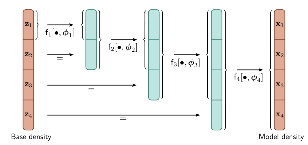
For the inverse process, the black arrows are reversed, and the last part of each block skips the remaining processing.

TODO

• Autoregressive flows, inverse autoregressive flows, residual flows,

Sources

• Prince, S. (2023). Understanding Deep Learning. Chapter 16.