Variational Autoencoders

Like normalizing flows, variational autoencoders or VAEs are probabilistic generative models; they aim to learn a distribution over the data. After training, it is possible to draw (generate) samples from this distribution. However, the properties of the VAE mean that it is not possible to evaluate the probability of new examples exactly.

It is common to talk about the VAE as if it is the model of , but this is misleading; the VAE is a neural architecture that is designed to help learn the model for . The final model for contains neither the variational nor the autoencoder parts and might be better described as a nonlinear latent variable model.

Latent Variable Models

Latent variable models take an indirect approach to describing a probability distribution over a multi-dimensional variable . Instead of directly writing the expression for , they model a joint distribution of the data and an unobserved latent variable . They then describe the probability as a marginalization of this joint probability so that

Typically, the joint probability is broken down using the rules of conditional probability into the likelihood of the data with respect to the latent variables term and the prior :

This is a rather indirect approach to describing , but it is useful because relatively simple expressions for and can define complex distributions .

Nonlinear Latent Variable Model

The previous section described the general latent variable decomposition

The nonlinear latent variable model turns this template into a concrete generative model by choosing specific forms for the two pieces: a prior over latent variables and a likelihood that maps latent variables back to data. The goal is to make each piece simple while allowing the marginalized distribution to be complex.

In this model, both the data and the latent variable are continuous and multivariate. The prior is a standard multivariate normal:

The likelihood is also normally distributed. Its mean is a nonlinear function of the latent variable, and its covariance is spherical:

When we need the value of a normal density at a particular point, we write this as , where the semicolon separates the value being evaluated from the distribution parameters.
The function is described by a deep neural network with parameters . This is what makes the model nonlinear: nearby or simple latent values can be mapped through a flexible neural network to complicated regions of data space. The latent variable is usually lower dimensional than the data , so describes the important structure in the data, and the remaining unmodeled variation is ascribed to the noise .

With these choices, the joint distribution factors into the same conditional form as before:

The data probability is then found by marginalizing over the latent variable :

Intuition

This can be viewed as an infinite weighted sum (i.e. an infinite mixture) of spherical Gaussians with different means, where the weights are and the means are the network outputs .

Generation

A new example can be generated using ancestral sampling. We draw from the prior and pass this through the network to compute the mean of the likelihood , from which we draw . Both the prior and likelihood are normal distributions, so this is straightforward.

Training

To train the model, we maximize the log-likelihood over a training dataset with respect to the model parameters. For simplicity, we assume that the variance term in the likelihood expression is known and concentrate on learning :

where

Caution

This objective is intractable. There is no closed-form expression for the integral and no easy way to evaluate it for a particular value of .

Evidence Lower Bound (ELBO)

The direct maximum likelihood objective fails because requires an intractable marginalization over . The integral combines the simple prior with the nonlinear decoder likelihood , whose mean is produced by a neural network. Because of this nonlinear transformation, there is generally no closed-form solution, and direct numerical integration becomes impractical when is high-dimensional. To make progress, we optimize a lower bound on the log-likelihood instead. This lower bound is always less than or equal to , and if the bound is close to the true log-likelihood, then improving the bound also improves the model.

To define this lower bound, we need Jensen’s Inequality and use the logarithm as the concave function:

or by writing out the expression for the expectation

Deriving the Bound

For a fixed observed data point , we introduce an arbitrary probability distribution over latent variables. This is not yet the encoder; it is just a distribution that lets us rewrite the marginal likelihood as an expectation:

We then use Jensen’s Inequality for the logarithm to find a lower bound:

where the right-hand side is termed the evidence lower bound or ELBO. It gets its name because is called the evidence in the context of Bayes Rule:

Eventually, will be replaced by a data-dependent, parameterized approximation :

The reason should depend on is that different data points should generally be explained by different regions of latent space. For each observed , we want a distribution over latent values that could plausibly have generated that particular example. In a VAE, this data-dependent distribution is produced by an encoder network with parameters . For now, can be understood as controlling the lower bound; later we will see that the encoder is used to approximate an intractable posterior distribution.

To learn the nonlinear latent variable model, we maximize this quantity as a function of both and . The neural architecture that computes this quantity is the VAE.

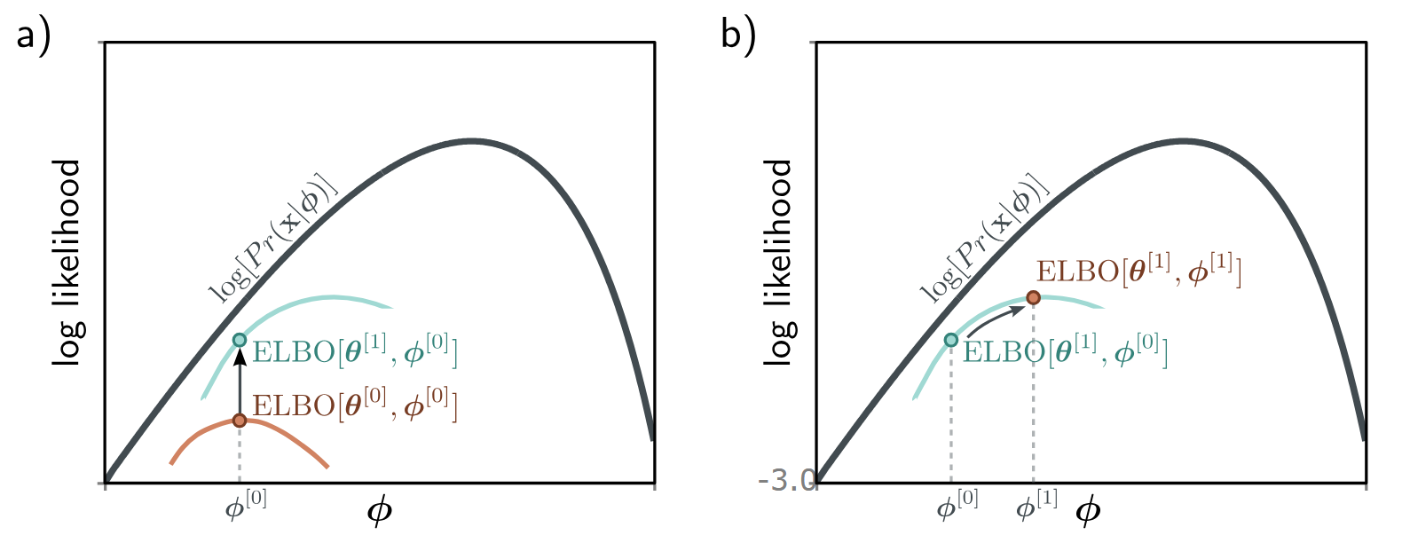
ELBO Properties

Consider that the original log-likelihood of the data is a function of the decoder parameters , and that we want to find its maximum. For any fixed encoder parameters , the ELBO is still a function of , but it must lie below the original log-likelihood function. When we change , we change the lower bound itself, and the bound may move closer to or further from the log-likelihood. When we change , we move along the current lower bound.

The figure below separates these two effects: the left graph shows how changing can move the lower bound upward for a fixed , while the right graph shows how changing moves along the lower bound.

Two Views of the Same ELBO

The ELBO can be rewritten in two useful ways depending on how we factor the joint distribution . These are not two different objectives; they are two interpretations of the same lower bound.

If we factor the joint as

then the ELBO becomes the true log-likelihood minus a KL divergence to the true posterior. This view explains why the bound is lower than the log-likelihood and when it becomes tight.

If we factor the joint as

then the ELBO becomes a reconstruction term minus a KL divergence to the prior. This view explains the training objective used by the VAE: decode latent samples that explain well, while keeping the encoder distribution close to the prior used for generation.

Intuition

The first view compares the ELBO to the quantity we wish we could optimize directly, . The second view shows how to compute and optimize the bound in practice. The first view answers “how good is the bound?” The second view answers “what pressure does the VAE training objective put on the encoder and decoder?”

Tightness of Bound

The ELBO is tight when, for a fixed value of , the ELBO and the log-likelihood function coincide. To find the distribution that makes the bound tight, we factor the numerator of the log term in the ELBO using the definition of conditional probability:

Here, the first integral disappears between lines three and four since does not depend on , and the integral of the distribution is one. In the last line, we used the definition of the Kullback-Leibler Divergence.

Intuition

The ELBO is the original log-likelihood minus the KL divergence between and the true posterior . This KL divergence is the gap between the lower bound and the true log-likelihood. The KL will be zero, and the bound tight, when . This true posterior indicates which latent values could have been responsible for the observed data point.

Caution

This form explains the bound, but it cannot be used directly for training. It contains both and the true posterior , and both require the same intractable marginal likelihood . This motivates rewriting the same ELBO in terms of the decoder likelihood and the prior.

ELBO as Reconstruction Term Minus KL to Prior

A second useful way to express the same ELBO is as a reconstruction term minus the distance to the prior:

where the joint distribution has been factored into conditional probability between the first and second lines, and the definition of the KL divergence is used in the last line.

Why This Form Helps

This version no longer contains the true posterior or the marginal likelihood explicitly. It uses the decoder likelihood , the prior , and the chosen encoder distribution , which are terms we can compute, sample from, or approximate.

Intuition

The first term measures the average agreement between the observed data and the decoder likelihood , where the average is taken over latent values sampled from . This is a reconstruction term because is chosen to put probability mass on latent values that plausibly explain this particular ; for each such , the decoder is rewarded when it assigns high probability to reconstructing the same . The average is not taken over the prior because the prior describes how to generate new latent variables before seeing any data, while is the data-dependent distribution over latent variables after seeing . The second term measures the degree to which matches the prior. When training by minimizing the negative ELBO, the first term becomes a reconstruction loss and the second term becomes a KL penalty.

Why Return to the Posterior View?

The reconstruction/prior form does not explicitly contain the true posterior , but it is still the same ELBO. This means the best possible choice of has not changed. If we were allowed to choose any distribution for , the distribution that maximizes the ELBO would still be the true posterior.

The posterior view tells us what is trying to approximate. The reconstruction/prior view tells us how to train the model without explicitly evaluating that posterior. In other words, the true posterior is the ideal target for the encoder distribution, while the reconstruction term and KL-to-prior term are the practical signals used to learn it.

Variational Approximation

Problem: Intractable Posterior

The tightness result says that the best possible choice for is the true posterior . This is why we return to the posterior view before defining the encoder approximation. In principle, we can compute this posterior using Bayes Rule:

but in practice this is intractable because we cannot evaluate the term in the denominator. This is the same marginal likelihood that caused the original training problem.

• is the prior; how plausible was this latent code before seeing
• is the decoder likelihood; if this were the latent code, how likely would it be to produce the observed
• is the posterior; after seeing , how plausible is this latent code as its explanation

Solution: Variational Family

The solution is to make a variational approximation: we choose a simple parametric family for and use this to approximate the true posterior. Here, we choose a multivariate normal distribution with mean and covariance :

where is a second neural network with parameters that predicts the mean and covariance of the normal variational approximation.

This Gaussian family will not always match the true posterior perfectly, but it may be a good approximation for some values of and . We do not directly minimize the KL divergence to the true posterior because the true posterior is unavailable. Instead, we maximize the ELBO, which indirectly pushes toward while also improving the decoder parameters .

Intuition

This is not a coincidence: the posterior view tells us the ideal target for , while the reconstruction/prior view gives a tractable objective that pushes toward that target.

Amortized Inference

This also explains why we use an encoder network. In principle, each data point could have its own variational parameters and , but then inference would require solving a separate optimization problem for every new . Instead, the VAE amortizes inference: a single network maps each data point to the parameters of its approximate posterior .

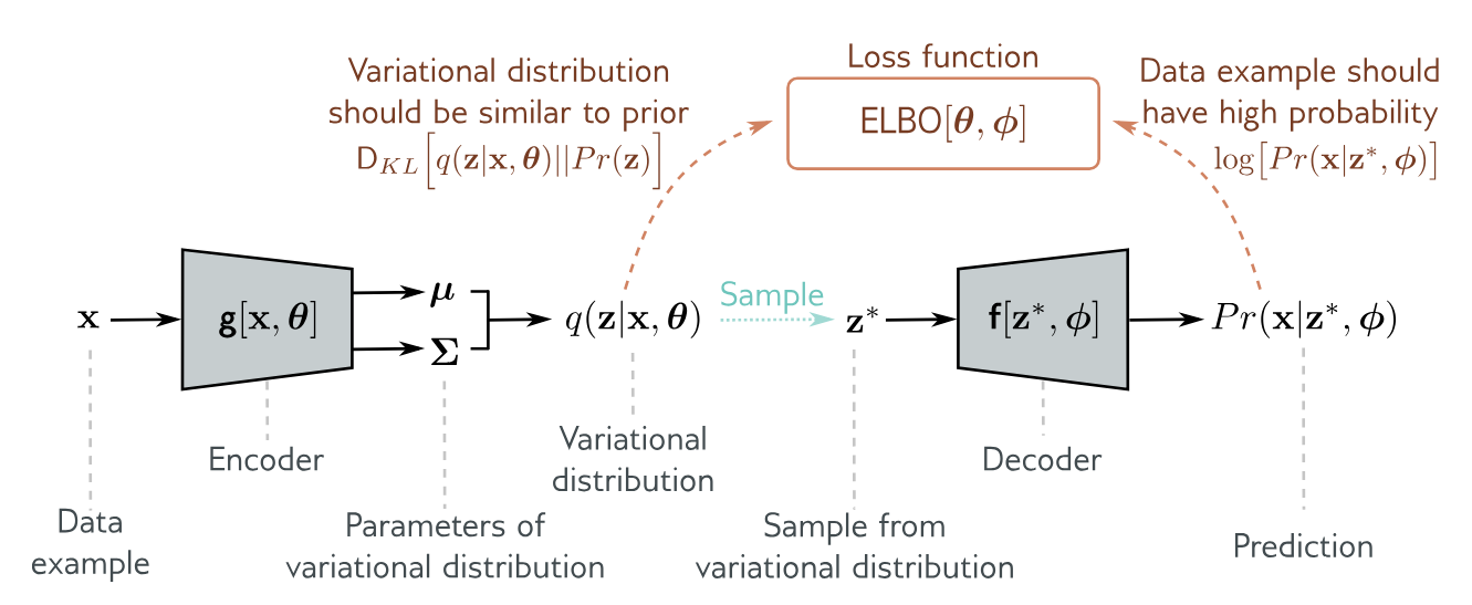
The Variational Autoencoder

With this variational approximation, the per-data-point ELBO is

The first term uses the encoder distribution to choose latent values that should reconstruct the current data point well. The second term keeps those data-dependent latent distributions close to the prior , which is the distribution used later for generation.

Monte Carlo Estimate

Caution

The first term still involves an intractable integral, but since it is an expectation with respect to , we can approximate it by sampling.

For any function we have

where is the th sample from . This is known as a Monte Carlo estimate. In practice, VAEs often use a single sample from :

The second term is the KL divergence between the variational distribution and the prior . The KL divergence between two normal distributions can be calculated in closed form:

where is the dimensionality of the latent space.

Reparameterization Trick

Caution

Sampling solves the intractable expectation, but it introduces a new problem: the sample is drawn from a distribution whose parameters come from the encoder. If the sampling operation is treated as an opaque random step, gradients from the reconstruction term cannot flow cleanly back through , , and .

Definition (Reparameterization Trick)

The solution is to move the stochastic part into a parameter-free noise variable. First draw

and then construct

The randomness now comes from , while is a differentiable function of the encoder outputs and . For a diagonal covariance, this is usually written as .

VAE Algorithm

To summarize, the VAE computes an approximate ELBO for each data point and uses an optimization algorithm to maximize this lower bound over the dataset. For a point , the steps are:

1. Use the encoder to compute the mean and covariance of .
2. Draw parameter-free noise .
3. Use the reparameterization trick to form .
4. Use the decoder to compute the likelihood .
5. Estimate the reconstruction term with .
6. Compute the KL term in closed form.
7. Maximize the ELBO, or equivalently minimize the negative ELBO.

In summary:

• It is variational because it computes a Gaussian approximation to the posterior distribution.
• It is an autoencoder because it starts with a data point , computes a lower-dimensional latent vector from this, and then uses this vector to recreate the data point as closely as possible.
• In this context, the mapping from the data to the latent variable by the network is called the encoder, and the mapping from the latent variable to the data by the network is called the decoder.
• The VAE computes the ELBO as a function of both and . To maximize this bound, we run minibatches of samples through the network and update these parameters with an optimization algorithm such as SGD or Adam. During this process, we are both moving between the colored curves in the ELBO diagram (changing ) and along them (changing ).
• After training, generation uses the prior , not the encoder. We sample and decode through .

Caution

Samples from vanilla VAEs are generally low-quality. This is partly because of the naive spherical Gaussian noise model and partly because of the Gaussian models used for the prior and variational posterior.

Tip

One trick to improve generation quality is to sample from the aggregate posterior rather than the prior:

The sum averages the encoder distributions over the dataset. It is not averaging sampled latent vectors , and it is not collapsing the dataset to one mean and covariance. Each term is one Gaussian component with its own mean and covariance, so the aggregate posterior is a mixture of Gaussians that may be more representative of the latent regions the decoder saw during training. To sample from it, choose a data point , encode it to get , then sample from that distribution.

Modern VAEs can produce high-quality samples, but only using hierarchical priors and specialized network architecture and regularization techniques. Diffusion models can be viewed as VAEs with hierarchical priors. These also create very high-quality samples.

Sources

• Prince, S. (2023). Understanding Deep Learning. Chapter 17.