Convolutional Networks

Convolutional layers are specialized network components which are mainly used for processing image data. Images have some properties that suggest the need for specialized model architecture

• They are high-dimensional. Hidden layers in fully connected networks that would process image inputs would be prohibitive in memory and compute costs to handle the number of weights
• Nearby image pixels are statistically related. Fully connected networks have no notion of nearby.
• The interpretation of an image is stable under geometric transformations (translation, etc.). A fully connected model must learn the patterns of pixels that signify a tree separately at every position.

Definition (Convolutional Neural Network)

A network predominantly consisting of convolution layers is known as a convolutional neural network or *CNN.

Invariance and Equivariance

Definition (Invariant)

A function of an image is invariant to a transformation if

In other words, the output of the function is the same regardless of the transformation . Networks for image classification should be invariant to geometric transformations of the image such as translation, rotation, flipping, or warping.

Definition (Equivariant or Covariant)

A function of an image is equivariant or covariant to a transformation if

In other words, is equivariant to the transformation if its output changes in the same way under the transformation as the input. Networks for per-pixel image segmentation should be equivariant to transformations; if the image is translated, rotated, or flipped, the network should return a segmentation that has been transformed in the same way.

Convolutional Networks for 1D Inputs

Definition (Convolutional Layer)

Convolutional layers are network layers based on the convolution operation. In 1D, a convolution transforms an input vector into an output vector so that each output is a weighted sum of nearby inputs. The same weights are used at every position and are collectively called the convolution kernel or filter. The size of the region over which inputs are combined is termed the kernel size. For a kernel size of three, we have

where is the kernel.

Notice that the convolution operation is equivariant with respect to translation. If we translate the input , then the corresponding output is translated in the same way.

Padding

The convolution equation begs the question of how to deal with the first output (where there is no previous input) and the final output (where there is no subsequent input). There are two common approaches:

1. Pad the edges of the input with new values and proceed as usual. Zero-padding assumes the input is zero outside its valid range.
2. Discard the output positions where the kernel exceeds the range of the inputs. These valid convolutions have the advantage of introducing no extra information at the edges of the input. However, they have the disadvantage that the representation decreases in size.

Stride, Kernel Size, and Dilation

Convolution operations are a family, which are defined by the following attributes:

• Kernel Size/Filter Size: The dimension of the sliding window over the input. A larger kernel size can cover a larger spatial area of the input. It is typically kept as an odd number so that it can be centered around the current position
• Stride: How many inputs pixels the kernels should be shifted over at a time. If we have a stride of two, we create roughly half the number of outputs.
• Dilation Rule: The number of zeros interspersed between the weights plus one

Convolutional Layers

A convolutional layer computes its output by convolving the input, adding a bias , and passing each result through an activation function . With kernel size three, stride one, and dilation rate one, the th hidden unit would be computed as

which is a special case of a fully connected layer.

Channels

If we only apply a single convolution, information will likely be lost; we are averaging nearby inputs, and the ReLU activation function clips results that are less than zero. Hence, it is usual to compute several convolutions in parallel. Each convolution produces a new set of hidden variables, termed a feature map or channel.

In general, the input and hidden layers all have multiple channels. If the incoming layer has channels and we select a kernel size per channel, the hidden units in each output channel are computed as a weighted sum over all channels and kernel entries using a weight matrix and one bias. Hence, if there are channels in the next layer, then we need weights and biases.

Intuition

For each output channel, the spatial output is a linear combination of the inputs plus bias, passed through an activation function. This is repeated for each spatial output. Each output channel gives a new set of weights.

Receptive Fields

Definition (Receptive field)

The receptive field of a hidden unit in the network is the region of the original input that feeds into it.

For a stack of 1D convolutional layers with stride one, dilation one, and the same kernel size , the receptive field at layer is

This reflects that the first layer sees input positions, and each additional layer expands the receptive field by more positions.

Convolutional Networks for 2D Inputs

Convolutional layers can be applied to 2D image data. The convolutional kernel is now a 2D object.

If a kernel is size , and there are input channels, each output channel is a weighted sum of quantities plus one bias. It follows that to compute output channels, we need weights and biases.

For input , filters of size are applied to produce output , where

The weight tensor is of size which contains a filter transforming the channels to each channels.

Intuition

Without padding, the representation gets reduced in height and width for every convolution layer. As a result, the receptive field gets larger. Padding still results in the receptive field increasing at the same rate, but also allows the representation to remain the same size if chosen correctly.

Conv2D Implementation

Naive Implementation

Each thread computes a single element in the result tensor by performing a convolution over a tile of the input. A 3D grid block for each batch, output channels, and tile is launched, where each tile contains threads

constexpr int TW = 32;
 
template <typename T>
__global__ void conv_forward(
    const T *X, const T *W, T *Y,
    int W_grid, int C_in, int C_out, int H_in, int W_in,
    int K, int S, int P
) {
    int b = blockIdx.x;
    int m = blockIdx.y;
    int h = (blockIdx.z / W_grid) * TW + threadIdx.y;
    int w = (blockIdx.z % W_grid) * TW + threadIdx.x;
    const int H_out = (H_in + 2 * P - K) / S + 1;
    const int W_out = (W_in + 2 * P - K) / S + 1;
    T sum = 0;
 
    const int flat_size_in = C_in * H_in * W_in;
    const int flat_size_out = C_out * H_out * W_out;
    const int idx_res = b * flat_size_out + m * (H_out * W_out) + h * (W_out) + w;
 
    for (int c = 0; c < C_in; ++c) {
        for (int p = 0; p < K; ++p) {
            for (int q = 0; q < K; ++q) {
                int h_in = S * h + p - P;
                int w_in = S * w + q - P;
                int idx_in = b * flat_size_in + c * (H_in * W_in) + (h_in * W_in) + w_in;
                int idx_w = (m * C_in * K * K) + (c * K * K) + (p * K) + q;
                T X_val = (h_in < 0 || w_in < 0 || h_in >= H_in || w_in >= W_in) ? 0 : X[idx_in];
                sum += X_val * W[idx_w];
            }
        }
    }
    Y[idx_res] = sum;
}
...
const int H_out = (H_in + 2 * P - K) / S + 1;
const int W_out = (W_in + 2 * P - K) / S + 1;
int W_grid = ceil_div(W_out, TW);
int H_grid = ceil_div(H_out, TW);
 
dim3 blockDim(TW, TW, 1);
dim3 gridDim(B, C_out, W_grid * H_grid);
conv_forward<<<gridDim, blockDim>>>(dev_X, dev_W, dev_Y, B, C_in, C_out, H_in, W_in, K, S, P);

Conv2D as Matrix Multiplication

A Conv2D can be implemented as a matrix multiplication. The weight tensor of shape is reshaped into a matrix of shape , where each row represents one output filter. The input tensor of shape is then unrolled into a matrix , where each column contains the entries from one receptive field. This operation is often referred to as im2col.

The matrix product therefore has shape

which can then be reshaped back into the output tensor.

Caution

While this method utilizes fast matrix multiplication kernels, it requires explicitly storing the unrolled matrix , which has entries instead of the original input entries. For stride one with roughly equal input and output spatial sizes, this is approximately a factor of more memory.

Downsampling and Upsampling

While we’ve seen that the representation size can decrease as it passes through convolution layers, there are additional layer types to scale down and up the representation

Downsampling

There are several ways to downsample a representation using convolutional layers

• We can sample every other position by using a stride of 2
• Max Pooling retains the maximum of the 2x2 input values
• Mean Pooling retains the average of the 2x2 input values

Upsampling

There are several ways to upsample a representation using convolutional layers:

• To double the resolution, one can duplicate all the channels at each spatial positions four times
• Max Unpooling will distribute the values to the positions they originated from
• Bilinear interpolation to fill in the missing values between points where we have samples
• Transposed Convolution has twice as many outputs as inputs, and each input contributed to three of the outputs.

Changing the Number of Channels

Sometimes we want to change the number of channels between one hidden layer and the next without further spatial pooling. This is usually so we can combine the representation with another parallel computation. To accomplish this, we apply a convolution with kernel size one. Each element of the output layer is computed by taking a weighted sum of all the channels at the same position. We can repeat this multiple times with different weights to generate as many output channels as we need. The associated weights have size .

Applications

Image Classification

Most methods reshape the input images to a standard size (say 224x224 RGB), and the output is a probability distribution over classes. Typically, convolution layers and pooling layers are interleaved with the spatial resolution decreasing and number of channels increasing. The representation is then reshaped/flattened, passed through fully connected layers, then a softmax to produce probabilities for each class.

Object Detection

The YOLO network rescales the input to a 448x448 RGB image and processes it with convolutional layers to produce a coarse 7x7 spatial grid of features. Each grid cell is responsible for objects whose center falls inside that cell, and the network predicts both class probabilities and a small fixed number of candidate bounding boxes per cell. Each bounding box is described by its center , width, height, and a confidence score, so the boxes can still have different sizes even though they come from the same 7x7 grid.

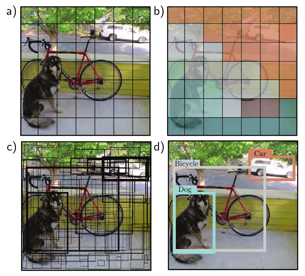
After prediction, low-confidence boxes are discarded and overlapping boxes for the same object are reduced using non-maximum suppression, leaving only the most confident detections.

Semantic Segmentation

The goal of segmentation is to assign a label to each pixel according to the object that it belongs to or no label if that pixel does not corresponding to anything in the training set. An example network passes the input image through convolutional layers, which reduce the spatial size but increase the number of channels. The representation is then flattened and passed into a fully connected layer. This then transformed back into a representation of size 7x7x512, and passed through max unpooling layers until the spatial shape matches the original input, but with channels representing one of each of the segmentation classes.

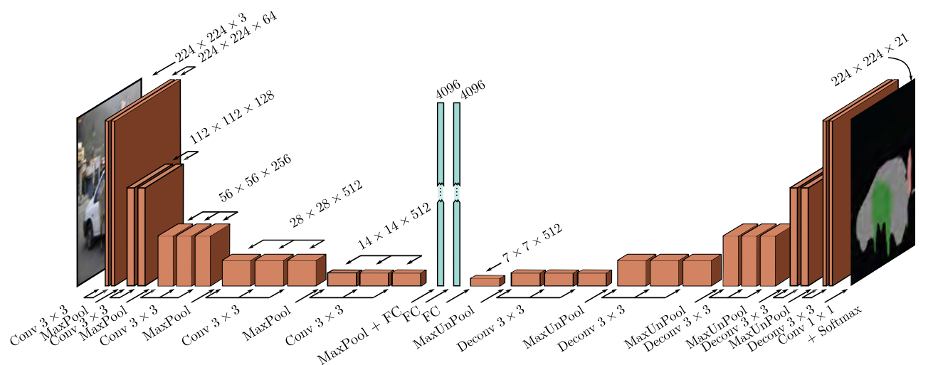
These two downscaling and upscaling models can be referred to as an encoder and decoder.

Additional Readings

• https://poloclub.github.io/cnn-explainer/
• YOLO Object Detection

Sources

• Prince, S. (2023). Understanding Deep Learning. Chapter 10.