Transformers
Transformer networks were initially targeted at natural language processing problems, where the network input is a series of high-dimensional embeddings representing words or word fragments. Language datasets share some characteristics of image data. The number of input variables can be very large, and the statistics are similar at every position; its not sensible to re-learn the meaning of the word dog at every possible position in a body of text. However, language datasets have the complication that text sequences vary in length, and unlike images, there is no easy way to resize them.
Processing Text Data
Consider the following sentence:
The restaurant refused to serve me a ham sandwich because it only cooks vegetarian food. In the end, they just gave me two slices of bread. Their ambiance was just as good as the food and service.
The goal is to design a network to process this text into a representation suitable for a downstream task, such as classify the review as positive or negative, or to answer questions about the restaurant. From this, we can see a few observations
- The encoded input can be very large. Each of the 37 words may be encoded into a 1024 representation embedding, resulting in an input of size
even for this small passage. Fully connected networks are impractical here - Each input is of a different length. Hence, it is not obvious how to apply a fully connected network. This suggests that the network should share parameters across words at different input positions, similar to convolutional networks share parameters across different image positions
- Language is ambiguous; it is unclear from syntax alone that the pronoun it refers to the restaurant and not the ham sandwich alone. To understand text, the word it should somehow be connected to the word restaurant. This implies there must be connections between the words and that the strength of these connections will depend on the words themselves.
Dot-Product Self-Attention
The transformer acquires the properties of (i) parameter sharing to cope with long input passages of differing lengths, and (ii) contain connections between word representations that depend on the word themselves, by using dot-product self-attention.
A standard neural network layer
where
Definition
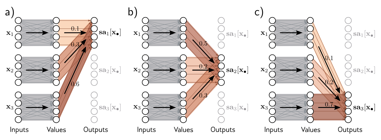
A self-attention block
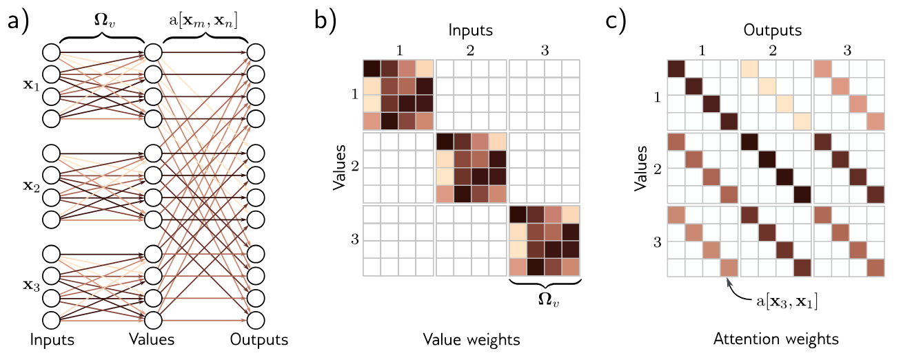
takes inputs , each of dimension , and returns outputs which are also of dimension . First, a set of values are computed for each input where
and represents biases and weights respectively. Then, the th output is a weighted sum of all the values :
The scalar weight
Computing and Weighting Values
The same weights
Intuition
The value computation can be viewed as a sparse matrix operation with shared parameters that relates these
quantities.
Computing Attention Weights
The attention weights are themselves nonlinear functions of the input. This is an example of a hypernetwork, where one network branch computes the weights of another. To compute attention, we apply two more linear transformations to the inputs:
where
so for each
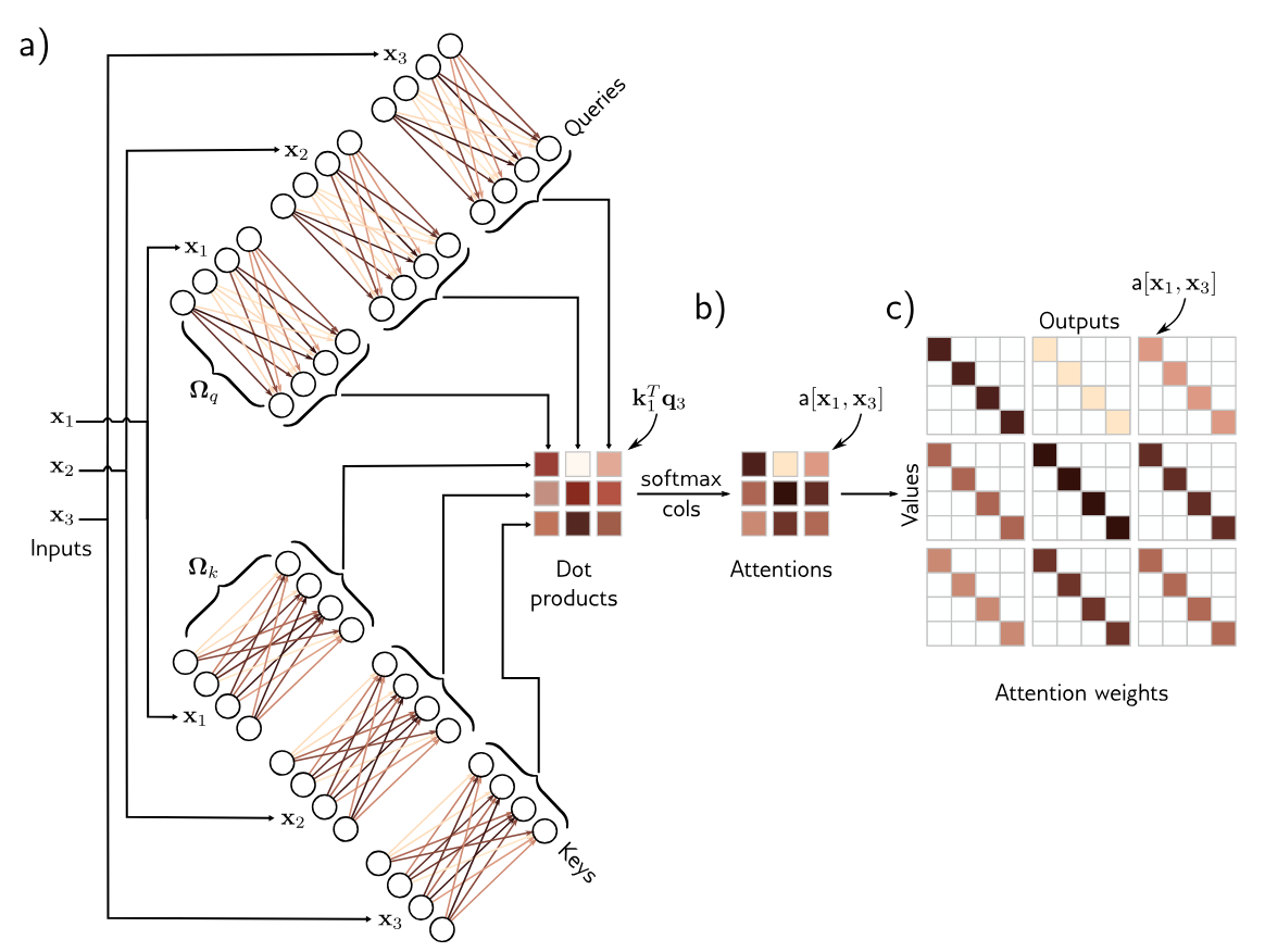
Matrix Form
The above computation can be written in a compact form if the
where
where the function
PyTorch Implementation
class SelfAttention(nn.Module):
    def __init__(self, embed_dim: int):
        super(SelfAttention, self).__init__()
        self.embed_dim = embed_dim

        # Projects for Q,K, and V
        self.query = nn.Linear(embed_dim, embed_dim)
        self.key = nn.Linear(embed_dim, embed_dim)
        self.value = nn.Linear(embed_dim, embed_dim)

    def forward(self, x: torch.Tensor, mask = None) -> torch.Tensor:
        # x: [batch_size, seq_len, embed_dim]
        Q = self.query(x)  # [batch_size, seq_len, embed_dim]
        K = self.key(x)    # [batch_size, seq_len, embed_dim]
        V = self.value(x)  # [batch_size, seq_len, embed_dim]

        # Dot product scores and scale
        scores = torch.matmul(q, k.transpose(-2, -1))
                    / (self.embed_dim ** 0.5)     # [batch_size, seq_len, seq_len]

        # Optional masking
        if mask is not None:
            scores = scores.masked_fill(mask == 0, -10000)

        # Attention weights
        attn_weights = F.softmax(scores, dim=-1)  # [batch_size, seq_len, seq_len]

        return torch.matmul(attn_weights, V)      # [batch_size, seq_len, embed_dim]
The scaling of the scores prevents the dot product from growing with dimension, avoiding softmax saturation and improving gradient flow during training. The
Extensions to Dot-Product Self-Attention
Positional Encoding
The self-attention mechanism computation does not take into account the order of the inputs
- Absolute Positional Encodings: A matrix
is added to the input that encodes positional information. Each column of is unique and hence contains information about the absolute position in the input sequence. This matrix can be chosen by hand or learned. It may be added to the network inputs or at every network layer. Sometimes it is added to in the computation of the queries and keys but not the values. - Relative Positional Encoding: Sometimes the absolute position of a word is less important than the relative position between two words. Each element of the attention matrix corresponds to a particular offset between key position
and query position . Relative positional encoding learns a parameter for each offset and use this to modify the attention matrix by adding these values, multiplying by them, or using them to alter the attention matrix in some other way.
Rotary Positional Embeddings (RoPE)
Rotary positional embeddings (RoPE) are a common modern way to add position information to transformer models, especially decoder-only language models. Instead of adding a learned positional vector to the token embedding, RoPE applies a position-dependent rotation to the queries and keys before computing attention.
For a query at position
where
This solves the positional encoding problem by making the attention score depend on the relative displacement between positions. In other words, the model can learn patterns like “attend to the previous token”, “attend to something ten tokens ago”, or “attend to distant context”, rather than only learning that a token occurs at an absolute position such as 137.
RoPE is also useful for long-context transformers. With learned absolute positional embeddings, a model trained on sequences of length 2048 has only learned embeddings for those positions, so extending it to much longer contexts is awkward. RoPE does not require a separate learned vector for each possible position. Its rotations are generated from a formula, so they can be evaluated at positions beyond the original training length. This does not automatically make a short-context model perfect at long-context reasoning, but it makes the architecture much easier to adapt using techniques such as RoPE scaling, interpolation, and long-context fine-tuning.
Intuition
RoPE is both a positional encoding method and an enabler for long-context adaptation. It gives the model relative position information while avoiding a fixed learned table of absolute positions.
Scaled Dot-Product Self-Attention
The dot products in the attention computation can have large magnitudes and move the arguments to the softmax function into a region where the largest value completely dominates. Small changes to the inputs to the softmax function now have little effect on the output (i.e. the gradients are very small), making the model difficult to train. To prevent this, the dot products are scaled by the square root of the dimension
Definition (Scaled dot-product self-attention)
Scaled dot-product self-attention is given by
Multiple Heads
Definition (Multi-Head Self-Attention)
Multiple self-attention mechanisms are usually applied in parallel, and this is known as multi-head self-attention. Now,
different sets of values, keys, and queries are computed: The
th self-attention mechanism or head can be written as where we have different parameters for each head.
Typically, if the dimension of the inputs
This choice makes sense for several reasons:
- The total width across all heads remains
, so concatenating the head outputs returns to the original model dimension. - The query, key, and value projections still map from width
to total width , so using multiple heads does not substantially increase the parameter count compared with a single width- attention block. - Each head computes dot products in a smaller
dimensional subspace, so the work per head is reduced, while the total work across all heads remains of the same order as single-head attention. - Different heads can specialize to different learned subspaces of the representation without increasing the overall representation size.
The outputs of these self-attention mechanisms are vertically concatenated, and another linear transform
Caution
Multiple heads seem to be necessary to make self-attention to work well. It has been speculated that they make the self-attention network more robust to bad initializations.
Implementation Note
In the mathematical description, each head
has its own parameters . In code, these are usually not implemented as completely separate nn.Linearmodules. Instead, each projection is packed into a single linear layer of shape, where the output dimension is interpreted as contiguous blocks of size . For example, if the model dimension is
and there are heads, then each head has width . A single query projection maps each token from shape [512]to shape[512], but that 512-dimensional output is then reshaped into[8, 64]. The first 64 entries correspond to head 1, the next 64 to head 2, and so on. The same idea is used for keys and values.So conceptually we still have
different sets of weights, but they are stored inside one larger weight matrix rather than as separate PyTorch layers. If we wrote the query matrix as then applying this single matrix computes all head-specific queries at once, after which we simply reshape the result to split out the head dimension. This is mathematically equivalent to running
separate attention heads, but is much more efficient because the implementation can use a small number of large batched matrix multiplies instead of many smaller ones.
PyTorch Implementation
class MultiHeadAttention(nn.Module):
    def __init__(self, embed_dim: int, num_heads: int):
        super(MultiHeadAttention, self).__init__()
        assert embed_dim % num_heads == 0, "embed_dim must be divisible by num_heads"

        self.embed_dim = embed_dim
        self.num_heads = num_heads
        self.head_dim = embed_dim // num_heads

        # Project to the concatenated Q, K, and V representations for all heads.
        self.query = nn.Linear(embed_dim, embed_dim)
        self.key = nn.Linear(embed_dim, embed_dim)
        self.value = nn.Linear(embed_dim, embed_dim)

        # Combine the concatenated head outputs back into the model dimension.
        self.out = nn.Linear(embed_dim, embed_dim)

    def forward(self, x: torch.Tensor, mask = None) -> torch.Tensor:
        # x: [batch_size, seq_len, embed_dim]
        batch_size, seq_len, _ = x.shape

        Q = self.query(x)  # [batch_size, seq_len, embed_dim]
        K = self.key(x)    # [batch_size, seq_len, embed_dim]
        V = self.value(x)  # [batch_size, seq_len, embed_dim]

        # Reshape to [batch_size, num_heads, seq_len, head_dim].
        # The transpose moves num_heads before seq_len so attention
        #   is computed independently per head.
        Q = Q.view(batch_size, seq_len, self.num_heads, self.head_dim)
             .transpose(1, 2)    # [batch_size, num_heads, seq_len, head_dim]
        K = K.view(batch_size, seq_len, self.num_heads, self.head_dim)
             .transpose(1, 2)    # [batch_size, num_heads, seq_len, head_dim]
        V = V.view(batch_size, seq_len, self.num_heads, self.head_dim)
             .transpose(1, 2)    # [batch_size, num_heads, seq_len, head_dim]

        # Scaled dot-product attention for each head.
        scores = torch.matmul(Q, K.transpose(-2, -1))
                    / (self.head_dim ** 0.5)  # [batch_size, num_heads, seq_len, seq_len]

        # Optional masking
        if mask is not None:
            scores = scores.masked_fill(mask == 0, -10000)

        # Attention weights
        attn_weights = F.softmax(scores, dim=-1)  # [batch_size, num_heads, seq_len, seq_len]

        head_outputs = torch.matmul(attn_weights, V)  # [batch_size, num_heads, seq_len, head_dim]

        # Concatenate heads back to [batch_size, seq_len, embed_dim].
        head_outputs = head_outputs.transpose(1, 2).contiguous()
                                   .view(batch_size, seq_len, self.embed_dim)

        return self.out(head_outputs)  # [batch_size, seq_len, embed_dim]
Transformer Layers
Self-attention is just one part of a larger transformer layer. This consists of a multi-head self-attention unit (which allows the word representations to interact with each outer) followed by a fully connected network
Definition (Transformer Layer)
The complete transformer layer can be described by the following series of operations:
where the column vectors
are separately taken from the full data matrix .
PyTorch Implementation
The feed-forward network is indeed just a small MLP applied to the last dimension of the tensor. If x has shape [batch_size, seq_len, embed_dim], then nn.Linear(embed_dim, hidden_dim) is applied independently to each token position, producing [batch_size, seq_len, hidden_dim]. This is why the feed-forward block is often called point-wise: it mixes features within each embedding vector, but does not mix information across different sequence positions.
class TransformerLayer(nn.Module):
    def __init__(self, embed_dim: int, num_heads: int, ffn_dim: int):
        super(TransformerLayer, self).__init__()
        self.attention = MultiHeadAttention(embed_dim, num_heads)
        self.norm1 = LayerNorm(embed_dim)
        self.ffn = nn.Sequential(
            nn.Linear(embed_dim, ffn_dim),
            nn.ReLU(),
            nn.Linear(ffn_dim, embed_dim),
        )
        self.norm2 = LayerNorm(embed_dim)

    def forward(self, x: torch.Tensor, mask = None) -> torch.Tensor:
        # x: [batch_size, seq_len, embed_dim]
        out = self.attention(x, mask) + x    # [batch_size, seq_len, embed_dim]
        out = self.norm1(out)                # [batch_size, seq_len, embed_dim]
        out = out + self.ffn(out)            # [batch_size, seq_len, embed_dim]
        out = self.norm2(out)                # [batch_size, seq_len, embed_dim]
        return out
Transformers for Natural Language Processing
A typical NLP pipeline stats with a tokenizer that splits the text into words or fragments. Then each of these tokens is mapped to a learned embedding. These embeddings are passed through a series of transformer layers.
Tokenization
Definition (Tokenizer)
A tokenizer splits the text into smaller units (tokens) from a vocabulary of possible tokens.
There are several difficulties with tokenizers:
- Inevitably, some words (e.g. names) will not be in the vocabulary
- Its unclear how to handle punctuation, but this is important. I fa sentence ends in a question mark, we must encode this information
- The vocabulary would need different tokens for versions of the same word with different suffixes (e.g. walk, walks, walked, walking, etc.), and there is no way to clarify that these are related.
In practice, a comprise is made between letters and full words is used, and the final vocabulary includes both common words and word fragments form which larger and less frequent words can be composed of. The vocabulary is computed using a sub-word tokenizer such as byte pair encoding that greedily merges commonly occurring sub-strings based on their frequency.
For example, a tokenizer might keep common whole words like the and play, but also common fragments like er and ing. Then the word playing might be tokenized as [play, ing], while a rarer word like player might be tokenized as [play, er]. This lets the model reuse frequent sub-word pieces instead of needing a completely separate vocabulary entry for every full word.
Embeddings
Each token in the vocabulary
Transformer Model
The embedding matrix
- An encoder transforms the text embeddings into a representation that can support a variety of tasks
- A decoder predicts the next token to continue the input text
- Encoder-Decoders are used in sequence-to-sequence tasks, where one text string is converted into another.
Encoder Model Example: BERT
BERT is an encoder model that uses a vocabulary 30,000 tokens. Input tokens are converted to 1024-dimensional word embeddings and passed through 24 transformer layers.
- Each contains a self-attention mechanism with 16 heads
- The queries, keys, and values for each head are of dimension 64 (i.e.
are ) - The dimension of the single hidden layer in the fully connected networks is 4096.
- The total number of parameters is ~340 million.
Encoder models like BERT exploit transfer learning. During pre-training, the parameters of the transformer architecture are learned using self-supervision from a large corpus of text. The goal here is for the model to learn general information about the statistics of the language. In the fine-tuning stage, the resulting network is adapted to solve a particular task using a smaller body of labelled training data.
Pre-Training
In the pre-training stage, the network is trained using self-supervision. This allows the use of enormous amounts of data without the need for manual labels. For BERT, the self-supervision task consists of predicting missing words from sentences from a large internet corpus. During training, the maximum input length is 512 tokens, and the batch size is 256. The system is trained for a million steps, corresponding to roughly 50 epochs.
Predicting missing words forces the transformer network to understand some syntax. It also allows the model to learn superficial common sense about the world. For example, after training the model will assign a higher probability to the missing word train in the sentence The <MASK> pulled into the station.
Fine-Tuning
In the fine-tuning stage, the model parameters are adjusted to specialize the network to a particular task. An extra layer is appended onto the transformer network to convert the output vectors to the desired output. Examples include text classification, word classification, and text span prediction.
Decoder Model Example: GPT3
The basic architecture is similar to the encoder model and comprises a series of transformer layers that operate on learned word embeddings. However, the goal is different. The encoder aimed to build a representation of the text that could be fine-tuned to solve a variety of specific NLP tasks. Conversely, the decoder has one purpose: to generate the next token in the sequence. It can generate a coherent text passage by feeding the extended sequence back into the model.
Language Modeling
GPT3 is an autoregressive language model. Consider the sentence it takes create courage to let yourself appear weak. Assuming that tokens are individual words, the probability of the full sentence can be factored as
An autoregressive model predicts the conditional distribution
Masked Self-Attention
To train a decoder, we seek parameters that maximize the log probability of the input text under the autoregressive model (i.e. maximize that sum of the log conditional probability terms). Ideally, we would pass in the whole sentence and compute all the log probabilities and gradients int he same forward pass, rather than doing a forward pass for each token in the sentence.
Caution
If we pass in the full sentence, the term computing
would have access to both the answer greatand the right contextcourage to let yourself appear weak. Hence, the system can cheat rather than learn to predict the following words and won’t train propery.
Fix
The tokens only interact in the self-attention layers in a transformer network. Hence, the problem can be resolved by ensuring that the attention to the answer and the right context is zero. This can be achieved by setting the corresponding dot products (scores) in the self-attention computation to negative infinity before they are passed through the
function. This is known as masked self-attention.
The decoder operates as follows:
- The input text is tokenized and converted to embeddings
- The embeddings are passed into the transformer, and masked self-attention is used so that they can only attend to the current and previous tokens
- After the transformer layers, a single linear layer maps each output embedding to the size of the vocabulary, followed by a
function that converts these values to the probabilities
Generating Text from a Decoder
Since the autoregressive model defines a probability model over text sequences, it can be used to sample new examples of plausible text:
- To generate from the model, we start with an input sequence of text (which can just be the special
<START>token indicating the beginning of the sequence) and feed this into the network, which then outputs the probabilities over possible subsequent tokens - We can then either pick the most likely token or sample from this probability distribution, and append to the sequence that was fed into the network
- The new extended sequence can be fed back into the decoder network to yield the probability distribution over the next token
- By repeating this process, we can generate large bodies of text
Tip
The computation can be made quite efficient as prior embeddings do not depend on subsequent ones due to the masked self-attention. Hence, much of the earlier computation can be recycled as we generate subsequent tokens. For example, once the embeddings for the prefix tokens have been computed, they do not need to be recomputed from scratch. More importantly, at each transformer layer we can cache the keys and values for all previously generated tokens and only compute the new query/key/value for the latest token. Then the new token attends to the cached keys and values from the prefix rather than rerunning self-attention over the whole sequence. Similarly, the hidden states for earlier positions at intermediate layers are unchanged, so only the activations associated with the newest position need to be propagated through the stack of decoder layers.
In practice, many strategies can make the output text more coherent
- Beam search keeps track of multiple possible sentence completions to find the overall most likely sequence of words (which is not necessarily found by greedily choosing the most likely word at each step).
- Top-K sampling randomly draws the next word from only the top-K most likely possibilities to prevent the system from accidentally choosing from the long tail of low-probability tokens and leading to an unnecessary linguistic dead end.
More search-based decoding methods are discussed in Search-Based Decoding for Language Models.
GPT-3
- The sequence lengths are 2048 tokens long, and the total batch size is 3.2 million tokens
- There are 96 transformer layers (some of which implement a sparse version of attention), each processing a word embedding of size 12,288
- There are 96 heads in the self-attention layers, and the value/query/key dimension is 128
- It is trained with 300 billion tokens and contains 175 billion parameters
Encoder-Decoder Model Example: Machine Translation
Translation between languages is an example of a sequence-to-sequence task. One common approach uses both an encoder (to compute a good representation of the source sentence) and a decoder (to generate the sentence in the target language).
During training, the decoder receives the ground truth translation and passes it through a series of transformer layers that use masked self-attention and predict the following word at each position. However, the decoder layers also attend to the output of the encoder. This is achieved by modifying the transformer layers in the decoder. A new self-attention layer is added between the masked self-attention and neural network, in which the decoder embeddings attend to the encoder embeddings. This is called cross-attention, where the queries are computed from the decoder embeddings and the keys and values from the encoder embeddings.
Transformers for Long Sequences
Since each token in a transformer encoder model interacts with every other token, the computational complexity scales quadratically with the length of the sequence. For a decoder model, each token only interacts with the previous tokens, so there are roughly half the number of interactions, but the complexity still scales quadratically.
This quadratic increase in the amount of computation ultimately limits the length of sequences that can be used. Many methods have been developed to extend the transformer to cope with long sequences.
The move from GPT-3 style context lengths, such as 2048 tokens, to modern long-context models did not come from a single change. It came from combining several improvements:
- Memory-efficient exact attention: Methods such as FlashAttention compute the same attention operation as the vanilla transformer, but avoid materializing the full
attention matrix in slow GPU memory. Instead, the attention computation is tiled so that blocks of queries, keys, and values are loaded into fast on-chip memory. This does not change the arithmetic cost, but it greatly reduces memory usage and improves practical speed, making longer contexts feasible. - Sparse and local attention: Instead of letting every token attend to every previous token, each token may attend only to a local window, such as the previous 4096 tokens. This changes the cost from roughly
to where is the window size. Some models add a few global tokens or special attention patterns so important information can still travel across distant parts of the sequence. - Position encodings that extrapolate: A model trained with absolute positional embeddings for 2048 positions cannot automatically run at 128k positions, because it has no learned embeddings for those positions. Modern long-context models often use relative or rotary position encodings, such as RoPE, sometimes with interpolation or scaling tricks, so the model can represent positions beyond the length seen in the original training setup.
- KV-cache optimizations: During autoregressive generation, the keys and values for previous tokens are cached at every layer. For long contexts, this cache becomes very large. Variants such as multi-query attention and grouped-query attention reduce the number of key/value heads, so many query heads share the same cached keys and values. This does not remove the need to attend over the long prefix, but it makes inference memory much cheaper.
- Recurrence and external memory: Some architectures store compressed summaries or memory states from previous chunks of text. The current chunk can attend to this memory instead of attending to every previous token directly. This is useful when the full context is too long to represent explicitly with dense attention.
- Long-context training and fine-tuning: Even if the architecture can technically accept a long sequence, the model must be trained or fine-tuned on long examples to learn how to use distant context. Many long-context models are first trained at shorter lengths and then extended with a later stage of long-context training.
Hence, modern long-context transformers are usually not just vanilla GPT-3 scaled to a larger
Memory Pressure in Transformer Models
There are two different kinds of memory pressure in transformer models:
- Model memory: the memory required to store the learned parameters.
- Runtime memory: the memory required to store activations, attention intermediates, and cached keys/values during inference or training.
For the stored model footprint, the main drivers are the number of transformer layers, the model width, and the feed-forward network width. Each transformer layer contains attention projection weights for queries, keys, values, and the output projection, along with the feed-forward network. If the embedding dimension is
parameters per layer. A typical feed-forward network expands the embedding dimension to something like
parameters per layer. Hence, the feed-forward network often contains more parameters than the attention block itself.
The number of attention heads does not necessarily increase parameter memory if the model dimension
The input context size does not affect the stored parameter count. A model with a 2048-token context and a model with a 128k-token context can, in principle, have the same number of parameters. However, the context size has a large effect on runtime memory.
For autoregressive generation, a major runtime memory cost is the KV cache. At each layer, the model stores the keys and values for all previous tokens so they do not need to be recomputed at every generation step. The size of this cache scales roughly as
where
This is why methods like multi-query attention and grouped-query attention are useful. They reduce the number of key/value heads
Naive attention also creates an attention score tensor of shape [batch_size, num_heads, seq_len, seq_len], so its memory cost grows quadratically with sequence length. Memory-efficient exact attention methods such as FlashAttention reduce this pressure by avoiding materializing the full
Summary
The stored model size is mostly determined by the number of layers, the embedding dimension, and the feed-forward network width. The long-context inference memory cost is mostly determined by the KV cache, which scales with layers and context length. The number of heads matters most when it changes the total model width or the number of key/value heads.
Transformers for Images
The success of transformers on textual data led to experimentation on images. This was not obviously a promising idea for two reasons
- There are many more pixels in an image than words in a sentence, so the quadratic complexity of self-attention imposes a practical bottleneck.
- Convolutional nets have a good inductive bias because each layer is equivariant to spatial translation, and it takes into account the 2D structure of the image. However, this must be learned in a transformer network.
Regardless of these apparent disadvantages, transformer networks for images have now eclipsed the performance of convolutional networks for image classification and other tasks. This is partly because of the enormous scale at which they can be constructed and the large amount of data that can be used to pre-train networks.
The structural difference is that a convolutional layer applies the same local kernel at every spatial position. This is a strong and useful bias: it assumes that nearby pixels are most relevant and that the same feature detector should be useful everywhere in the image. However, it also means that long-range interactions must be built up gradually across many layers, as the receptive field expands.
In a vision transformer, the image is split into patches, and self-attention allows every patch to interact with every other patch in a single layer. This gives the model a global receptive field from the start. A patch corresponding to an object’s head can directly attend to a patch corresponding to its body, or a foreground object can directly attend to distant background context.
Another difference is that convolution uses a fixed spatial computation pattern: the same kernel is applied regardless of the image content. Attention is content-dependent. The attention weights are computed from the patches themselves, so the model can dynamically decide which regions are relevant for a particular image. In this sense, transformers can learn CNN-like local behavior when locality is useful, but they are not restricted to it.
Intuition
Convolutional networks have stronger built-in visual assumptions, which makes them data-efficient. Vision transformers have weaker assumptions, but more flexible global and content-dependent computation. With enough pre-training data and compute, this flexibility can outweigh the benefits of the convolutional inductive bias.
ImageGPT
ImageGPT is a transformer decoder; it builds an autoregressive model of image pixels that ingests a partial image and predicts the subsequent pixel value. The quadratic complexity of the transformer network means that the largest model could still only operate on
ImageGPT learns a separate positional encoding at each pixel. Hence, it must learn that each pixel has a close relationship with its preceding neighbor and also with nearby pixels in the row above. The internal representation of the decoder was used as a basis for image classification. Each pixel’s final embedding is averaged, and a linear layer maps these values to activations that pass through a softmax and predict class probabilities.
Despite using large amounts of external training data, the system achieve only a 27.4% top-1 error rate on ImageNet, which was worse than convolutional architectures at the time.
Vision Transformers (ViT)
The Vision Transformer tackled the problem of image resolution by dividing the image into 16x16 patches. Each patch is mapped to an input embedding via a learned transformation, and these representations are fed into the transformer. Once again, standard 1D positional encodings are learned.
This is an encoder model. Unlike BERT, it uses supervised pre-training on a large data base of 303 million labelled images. The <CLS> token is mapped via a final network layer to create activations that are fed into a softmax function to generate class probabilities. After pre-training, the system is applied to the final classification task by replacing this final alyer with one that maps to the desired number of classes an is fine-tuned.
Sources
- Prince, S. (2023). Understanding Deep Learning. Chapter 12.
- RoFormer: Enhanced Transformer with Rotary Position Embedding
- Position Information in Transformers: An Overview
- BERT: Pre-training of Deep Bidirectional Transformers for Language Understanding
- FlashAttention: Fast and Memory-Efficient Attention with IO-Awareness
- https://huggingface.co/docs/text-generation-inference/conceptual/flash_attention
- ImageGPT
- Vision Transformer (ViT)