Residual Network
Image classification tasks improved as the depth of convolutional networks were increased. However, performance started to decrease again many more layers were added. Residual networks introduced layers which computes an additive change to the current representation instead of transforming it directly. This allows deepener networks to be trained, but can also cause an exponential increase in the activation magnitudes at initialization. Batch normalization compensates for this, which centers an rescales the activations at each layer.
Sequential Processing
Feedforward networks process the data sequentially; each layer receives the previous layer’s output and passes the result to the next layer. In a standard neural network, each layer consists of a linear transformation followed by an activation function. In a convolutional network, each layer consists of a set of convolutions followed by an activation function. Since the processing is sequential, we can think of this network as a series of nested functions
Limitation of Sequential Planning
In principle, we can add as many layers as we want. However, its been observed that in applications like image classification, performance decreases again as further layers are added. This decrease in performance shows in both the training and testing sets.
One conjecture of this phenomenon is that right after initialization, the loss gradients change unpredictable when we modify parameters in early network layers. With appropriate initialization of the weights, the gradient of the loss with respect to these parameter values will be reasonable (i.e. no exploding or vanishing gradients). However, the derivative assumes an infinitesimal change in the parameter, whereas optimization algorithms use a finite step. any reasonable choice of step size may move to a place with a completely different and unrelated gradient (the loss landscape looks like an enormous range of tiny mountains rather than a single smooth structure that is easy to descend). Consequently, the algorithm doesn’t make progress in the way that it does when the loss function gradient changes more slowly.
This conjecture is supported by empirical observations of gradients in networks with a single input and output. Nearby gradients are correlated for shallow networks, but this correlation quickly drops to zero for deep networks. This is terms the shattered gradients phenomenon. Shattered gradients presumable arise because changes in early network layers modify the output in an increasingly complex way as the network becomes deeper. In the above example, the derivative of the output
When we change the parameters that determine
Residual Connections and Residual Blocks
Definition (Residual Connections, Skip Connections)
Residual or skip connections are branches in the computational path, whereby the input to each network layer
is added back to the output.
The previous example is defined as
where the first term on the right-hand side of each line is the residual connection. Each
Definition (Residual block)
Each additive combination of the input and the processed output is known as a residual block or residual layer.
If we write this as a single function, we get
We can think of this equation as unraveling the network, and the final output is a sum of the input and four smaller networks.
Interpretation
One interpretation is that residual connections turn the original network into an ensemble of these smaller networks whose outputs are summed to compute the result.
A complementary way of thinking about this residual network is that it creates sixteen paths with differing number of transformations between input and output.
In general, gradients through shorter paths will be better behaved. Since various short chains of derivatives will contribute to the derivative for each layer, networks with residual links suffer less from shattered gradients.
Order of Operations Inside Residual Blocks
The order of the operations inside residual blocks is important. The residual branch must contain a nonlinear activation function, otherwise the stacked block collapses to a linear map and depth buys us very little.
Post-Activation ResNet Block
In the original ResNet formulation, the conventional block is
where the residual branch typically has the form
which is often summarized as
The reasoning is as follows.
- The convolutions perform the learned linear transformations.
- Batch normalization keeps the activation scale controlled, which is especially important because repeated residual additions can otherwise cause the magnitude to grow with depth.
- The activation function is applied only on the residual branch before the addition, so the skip connection itself remains as close as possible to an identity map.
- The final activation after addition lets the next block receive a nonlinear representation.
Keeping the skip path simple is one of the main ideas behind residual networks. If the skip path is exactly the identity, then the block can always fall back to passing its input forward unchanged by driving the residual branch toward zero. This makes optimization easier, because each block only has to learn a correction to the current representation rather than an entirely new transformation.
Pre-Activation ResNet Block
Later work found that an even better ordering is often the pre-activation block:
with
or, more compactly,
In this design there is no activation immediately after the addition. This preserves a cleaner identity path for both the forward activations and backward gradients, and empirically it makes very deep residual networks easier to optimize.
If the input and output dimensions do not match, the skip path cannot be a literal identity. In that case it is common to use a projection, usually a
Deeper Networks with Residual Connections
Tip
Adding residual connections roughly doubles the depth of the network that can be practically trained before performance degrades.
However, we would like to increase the depth further. To understand why residual connections do not allow us to increase the depth arbitrarily, we must consider how the variance of the activations changes during the forward pass and how the gradient magnitudes change during the backward pass.
Exploding Gradients in Residual Networks
Caution
Without careful network parameter initialization, the magnitudes of the intermediate values during the forward pass can increase or decrease exponentially. Similarly, the gradients during the backward pass can explode or vanish as we move backward through the network. Hence, we initialize the network parameters so that the expected variance of the activations (forward pass) and gradients (backward pass) remains the same between layers. He initialization achieves this for ReLU activations.
Now consider a residual network. We do not need to worry about the intermediate values or gradients vanishing with network depth since there exists a path whereby each layer directly contributes to the network output. However, even if we use He initialization within the residual block, the values in the forward pass increase exponentially as we move through the network.
Consider that we add the result of the processing in the residual block back to the input. Each branch has some (uncorrelated) variability. Hence, the overall variance increases when we recombine them. With ReLU activations and He initialization, the expected variance is unchanged by the processing in each block. Consequently, when we recombine with the input, the variance doubles, growing exponentially with the number of residual blocks. This limits the possible network depth before floating point precision is exceeded in the forward pass. A similar argument applies to the gradients in the backward pass.
An approach to help deal with the exploding gradients is to use batch normalization.
Common Residual Architectures
ResNet
Residual blocks were first used in convolutional networks for image classification. The resulting networks are known as residual networks, or ResNet for short. In ResNets, each residual block contains a batch normalization operation, a ReLU activation function, and a convolutional layer. This is followed by the same sequence again before adding back to the input. Trial and error have shown that this order of operations works well for image classification.
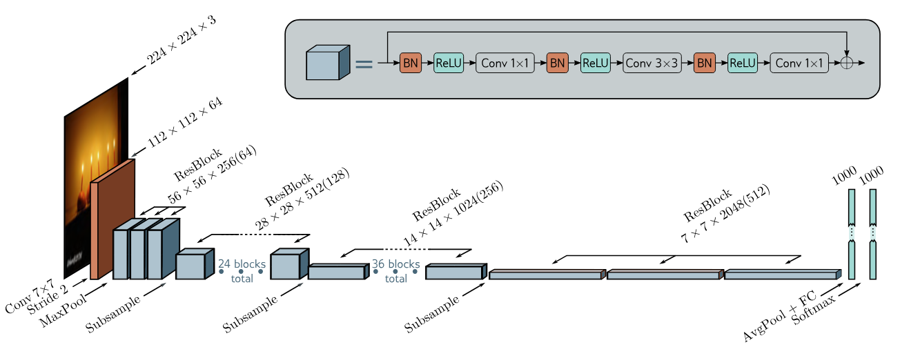
For very deep networks, the number of parameters may become undesirable large. Bottleneck residual blocks make more efficient use of parameters using three convolutions. The first has a 1x1 kernel and reduces the number of channels. The second is a regular 3x3 kernel, and the third is another 1x1 kernel to increase the number of channels back to the original amount. In this way, we can integrate information over a 3x3 pixel area using fewer parameters.
The resolution is decreased between adjacent ResNet blocks using convolutions of stride two. At the end, a fully connected layer maps the block to a vector of length 1,000, which is then passed through a softmax to generate class probabilities.
U-Net
In encoder-decoder networks for semantic segmentation, the encoder repeatedly downsamples the image until the receptive fields are large and information is integrated across the image. Then the decoder upsamples it back to the size of the original image. The final output is a probability over possible object classes at each pixel. The drawback is that the low-resolution representation in the middle of the network must remember the high-resolution details to make the final result accurate.
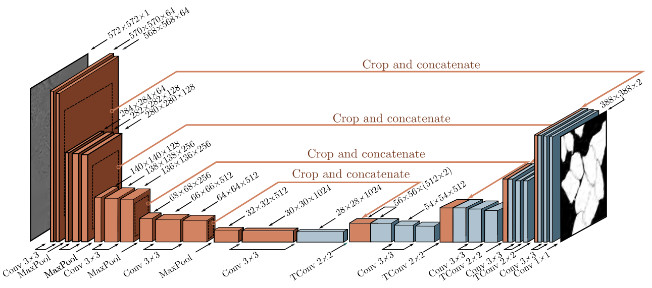
The U-Net is an encoder-decoder architecture where the earlier representations are concatenated to the later ones. The encoder uses regular convolutions, and the decoder uses transposed convolutions. Residual connections append the last representation at each scale in the encoder to the first representation at the same scale in the decoder. The original U-Net used valid convolutions, so the size decreased slightly with each layer, even without downsampling. Hence, the representations from the encoder were cropped before appending to the decoder.
Sources
- Prince, S. (2023). Understanding Deep Learning. Chapter 11.
- Deep Residual Learning for Image Recognition
- Identity Mappings in Deep Residual Networks
- U-Net: Convolutional Networks for Biomedical Image Segmentation
- ResNet strikes back: An improved training procedure in timm