Graph Neural Networks

As the name suggests , graph neural networks are neural architectures that process graphs (sets of nodes connected by edges). There are three novel challenges associated with processing graphs:

1. Their topology is variable, and its hard to design networks that are both sufficiently expressive and can cope with this variation.
2. Graphs may be enormous (billions of nodes).
3. There may only be a single monolithic graph available, so the usual protocol of training with many data examples and testing with new data is not always appropriate.

Graph Representations

A graph consists of a set of nodes connected by a set of edges. The graph can be encoded by three matrices , , and representing the graph structure, node embeddings, and edge embeddings respectively. The graph structure is represented by an adjacency matrix . This is an matrix where entry is set to one if there is an edge between nodes and and zero otherwise.

• The th node has an associated node embedding of length . These embeddings are concatenated and stored in the node data matrix .
• Similarly, the th edge has an associated edge embedding of length . These edges embeddings are collected into the matrix .

Properties of the Adjacency Matrix

Consider encoding the th node’s position as a one-hot column vector. When we pre-multiply this vector by the adjacency matrix, it extracts the th column of the adjacency matrix and returns a vector with ones a the position of the neighbors. If we repeat this procedure, the resulting vector contains the number of walks of length two from node . In general, if we raise the adjacency matrix to the power , the entry at position of contains the number of unique walks of length from node to node .

Caution

This is not the same as the number of unique paths since the walks include routes that visit the same node more than once.

Permutation of Node Indices

Node indexing in a graphs is arbitrary; permuting the node indices results in a permutation of the columns of the node data matrix and a permutation of both the rows and columns of the adjacency matrix .The operation of exchanging node indices can be expressed mathematically by a permutation matrix . This is a matrix where exactly one entry in each row and column take the value one, and the remaining entries are zero. When position of the permutation matrix is set to one, it indicates that node will become node after the permutation. To map one indexing to another, we use the operations:

where post-multiplying by permutes the columns and pre-multiplying by permutes the rows. It follows that any processing applied to the graph should also be indifferent to these permutations. Otherwise, it will depend on the choice of node indices.

Graph Neural Networks, Tasks, and Loss Functions

Definition

A graph neural network is a model that takes the node embedding and the adjacency matrix as inputs ans passes them through a series of layers. The node embeddings are updated at each layer to create intermediate hidden representations before finally computing the output embedding .

At the start of the network, each column of the input node embeddings just contains information about the node itself. At the end, each column of the mode output includes information about the node and its context within the graph. This is similar to word embeddings passing through a transformer network. These represent words at the start, but represent word meanings in the context of the sentence at the end.

Tasks and Loss Functions

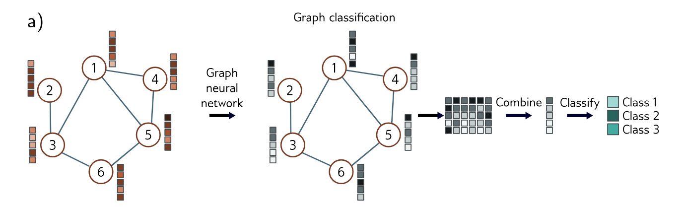
Graph-Level Tasks

The network assigns a label or estimates one or more values from the entire graph, exploiting both the structure and node embeddings. For example, we might want to predict the temperature at which a molecule becomes a liquid (regression task) or whether a molecule is poisonous to human beings or not (classification task).

For graph-level tasks, the output node embeddings are combined (by averaging), and the resulting vector is mapped via a linear transformation or neural network to a fixed-sized vector. For example, in binary classification, the output is passed through a sigmoid function, and the mismatch is calculated using the binary cross-entropy loss. Here, the probability that the graph belongs to class one might by given by

where the scalar and vector are learned parameters. Post-multiplying the output embedding matrix by the column vector that contains ones has the effect of summing together the embeddings, and subsequently dividing by the number of nodes computes the average.

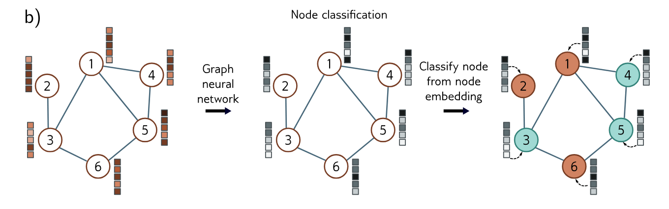
Node-Level Tasks

The network assigns a label (classification) or one or more values (regression) to each node of the graph, using both the graph structure and node embeddings. For example, given a graph constructed from a 3D point cloud, the goal might be to classify the nodes according to whether they belong to the wings or fuselage. Loss functions are defined in the same way as for graph-level tasks, except for now this is done independently for each node :

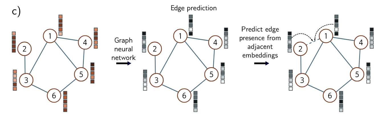
Edge Prediction Tasks

The network predicts whether or not there should be an edge between nodes and . For example, in the social network setting, the network might predict whether two people know and like each other and suggest that they connect if that is the case. This is a binary classification task where the two node embeddings must be mapped to a single number representing the probability that an edge is present. One possibility is to take the dot product of the node embeddings and pass the result through a sigmoid function to create the probability.

Graph Convolutional Networks (GCNs)

These models are convolutional in that they update each node by aggregating information from nearby nodes. As such, they induce a relational inductive bias (i.e. a bias towards prioritizing information from neighbors). They are spatial-based because they use the original graph structure.

Each layer of the GCN is a function with parameters that takes the node embeddings and adjacency matrix and outputs new node embeddings. The network can hence be written as

where is the input, is the adjacency matrix, contains the modified node embeddings at the th layer, and denotes the parameters that map from layer to layer .

Equivariance and Invariance

The indexing of the nodes in the graph is arbitrary, and any permutation of the node indices does not change the graph. It is hence imperative that any model respects this property. It follows that each layer must be equivariant with respect to permutation of node indices. If is a permutation matrix, then we must have that

For node classification and edge prediction tasks, the output should also be equivariant with respect to permutations of the node indices. However, for graph-level tasks, the final layer aggregates information from across the graph, so the output is invariant to the node order.

Parameter Sharing

Convolutional layers are applied to images that processed every position in the image identically. This reduced the number of parameters and introduced an inductive bias that forced the model to treat every part of the image in the same way. The same argument can be made about nodes in a graph. While in images we have a fixed-size square region around the current position when considering neighbors, in a graph each node may have a different number of neighbors, and there are no consistent relationships. There is no sense that we can weight information from a node that is above the node of interest differently to information from a node below it.

GCN Layer

These considerations lead to a simple GCN layer.

Definition

At each node in layer , we aggregate information from neighboring nodes by summing their node embeddings :

where returns the set of indices of the neighbors of node . Then we apply a linear transformation to the embedding at the current node and to this aggregated value, add a bias term , and pass the result through a nonlinear activation function , which is applied independently to every member of its vector argument:

We can write this more succinctly by noting that post-multiplication of a matrix by a vector returns a weighted sum of its columns. The th column of the adjacency matrix contains ones at the positions of the neighbors. Hence, if we collect the node embeddings into the matrix and post-multiply by the adjacency matrix , the th column of the result is . The update for the nodes is now

where is an vector containing ones and are the layer parameters. Here, the nonlinear activation function is applied independently to every member of its matrix arguments.

This satisfies the design considerations:

• it is equivariant to permutations of the node indices,
• can cope with neighbors,
• exploits the graph structure to provide a relational inductive bias,
• and shared parameters throughout the graph.

Training Considerations

Given training samples , each graph in a batch of samples may have a different number of nodes. Hence, the matrices and have different sizes, and there is no way to concatenate into a 3D tensor.

However, we can use the a trick by treating the graphs in the batch as disjoint components of a single large graph. The network can then be run as a single instance of the network equations.

Layers for Graph Convolutional Networks

The GCN combined messages from adjacent nodes by summing them together with the transformed current node. This was accomplished by post-multiplying the node embedding matrix by the adjacency matrix plus the identity . There are different approaches to both (i) the combination of the current embedding with the aggregated neighbors, and (ii) the aggregation process itself.

Combining Current Node and Aggregated Neighbors

Definition (Diagonal Enhancement)

In another variation, the current node is multiplied by a factor of before contributing to the sum, where is a learned scalar that is different for each layer:

This is known as diagonal enhancement. A related variation applied a different linear transform to the current node:

where .

Residual Connections

Definition (Residual Connections)

With residual connections, the aggregated representation from the neighbors is transformed and passed through the activation function before summation or concatenation with the current node. For the latter case, the associated network equations are

Mean Aggregation

The above methods aggregate the neighbors by summing the node embeddings. However, its possible to combine the embeddings in different ways. Sometimes its better to take the average of the neighbors rather than the sum. This can be superior if the embedding information is more important and the structural information less so since the magnitude of the neighborhood contributions will not depend on the number of neighbors.

Definition (Mean Aggregation)

Mean Aggregation is given by

where as before, denotes a set containing the indices of the neighbors of the th node. The above can be computed in matrix form by introducing the diagonal degree matrix . Each non-zero element of the matrix contains the number of neighbors for the associated node. It follows that each diagonal element in the inverse matrix contains the denominator that we need to compute the average. The new GCN layer can be written as

Kipf Normalization

There are many variations of graph neural networks based on mean aggregation. Sometimes the current node is included with its neighbors in the mean computation rather than treated separately.

Definition (Kipf Normalization)

In Kipf normalization, the sum of the node representations is normalized as

with the logic that information coming from nodes with a very large number of neighbors should be down-weighted since there are many connections and they provide less unique information. This can also be expressed in matrix form using the degree matrix:

Max Pooling Aggregation

An alternative operation that is invariant to permutation is computing the maximum of a set of objects.

Definition (Max Pooling Aggregation)

The max pooling aggregation operator is

where the operator returns the element-wise maximum of the vectors that are neighbors to the current node .

Aggregation by Attention

The aggregation methods discussed so far either weight the contribution of the neighbors equally or in a way that depends on the graph topology. Conversely, in graph attention layers, the weights depend on the data at the nodes.

Definition (Graph Attention Layer)

A linear transform is applied to the current node embeddings so that

Then the similarity of each transformed node embedding to the transformed node embedding is computed by concatenating the pairs, taking a dot product with a column vector of learned parameters, and applying an activation function

These variables are stored in an matrix , where each element represents the similarity of every node to every other. As in dot-product self attention, the attention weights contributing to each other embedding are normalized to be positive and sum to one using the softmax operation. However, only those values corresponding to the current node and its neighbors should contribute. The attention weights are applied to the transformed embeddings:

where is a second activation function. The function computes the attention values by applying softmax operation separately to each column of its first argument , but only after setting values where the second augment is zero to negative infinity, so they do not contribute. This ensures that the attention to non-neighboring nodes is zero.

This is similar to the dot-product self-attention computation in transformers, except that:

• The keys, queries, and values are all the same
• The measure of similarity is different
• The attentions are masked so that each node only attends to itself and its neighbors.

As in transformers, this system can be extended to use multiple heads that are run in parallel and recombined.

Sources

• Prince, S. (2023). Understanding Deep Learning. Chapter 13.
• Graph Attention Networks